Effective decision-making depends heavily on the quality of the data at available. In this blog, we will delve into six core dimensions of data quality with functional examples as well as basic MSSQL queries to develop better insights into your data.
What is Data Quality?
Data Quality (DQ) is the assessment of usefulness and reliability of data for its purpose. This process is often referred to as Data Profiling: a subjective discovery to understand your data and its usability relative to the standards defined by the user.
Example of Subjective Data Quality
A financial controller needs to know every decimal and cent in the data for it to be accurate. The sales department only needs approximated sales numbers to determine sales trends.
Partly intertwined are the processes of Data Integration (DI) and Master Data Management (MDM), which together is sometimes called Data Cleansing. This involves resolving and managing issues, standardizing data, enrichment and integrating various sources into a data system with the goal of unlocking full value, high-quality data.
Data Quality Metrics
In 2020 the Data Management Association (DAMA) compiled a list of 65 dimensions and subdimensions for Data Quality, with 12 of these being marked as ‘common’. Out of these twelve there are 6 core dimensions:
- Completeness:
— The main features required for analysis do not have missing values. - Uniqueness:
— Check that there is only one record of each observation in the data. - Timeliness and Currency:
— Data must be up to date and the most recent record reflects the most recent change. - Consistency:
— Minimize or remove contradictions within a dataset or between datasets. - Validity:
— Ensures data has the right type, format and is within acceptable range. - Accuracy:
— Measures the correctness of the form and content of data.
Managing Data Quality
Data Governance is a data management concept concerning the capability of a business to ensure high data quality exists during the lifecycle of the data, and that controls are in place that support business objectives.
In Data Governance the responsibility is skewed mostly towards business users and not to the IT infrastructure. While data is expected to be fixed at creation, it is often not assessed until it is consumed. That is why analysts are often burdened with the added task of detecting and resolving issues and flaws in the data.
This has led to a new role to centralize this responsibility: the Data Steward. A Data Steward is tasked with administering all data in compliance with policy and regulation. This role is often taken on by a Data Analyst or Data Scientist connected to the project or organization.
COMPLETENESS
Completeness is measured by the ratio of missing records for the features that are within the scope of the project. A completeness of 95% would mean that only 5 out of 100 records have missing values.
A real-world example:
At the cash register in the grocery store all products are scanned with a barcode on the packaging. For one of your items the barcode is missing, thus it cannot be registered for payment. The item is manually processed by the cashier, looking up the item code or price.
This manual involvement is surprisingly like how completeness is handled in business. Only when the salesperson tries to send an email to a customer the system returns a message that the email address isn’t available. They manually resolve the issue, either by getting the data from another system or by calling the customer to retrieve the missing email address.
Below an example of a basic test on the completeness of a table in a MSSQL database:
SELECT
100 * COUNT(CASE WHEN col A is not null THEN 1 END) / COUNT(*) AS completeness_col_A
FROM table_name
There are several options to resolve missing data and improve the overall completeness of your dataset. We’ve listed some of the solutions below:
- If available, use other data sources. This is a great solution for standardized data such as addresses and can be seen in online shopping. They only ask for your postal code and house number, which is used to retrieve the correct street name. A solution like this requires time to test external data sources and determine if they can be used to complete empty records or fields.
- Imputation is inferring the missing values from the existing ones, for example by replacing the missing values with the median, mean or mode of the data. Imputation does require a very clear definition of the goal and the precision of data needed.
An example in MSSQL:SELECT COALESCE (col_A, AVG (col_A) ) FROM table_name
- Manually fixing values, although possible and quite often common practice, is an undesirable solution. When the number of missing values is very low, and the business logic is well known, this is sometimes used as a quick fix. But the major downside manual resolution is non-scalability and human error.
- Dropping missing values is an option when the dataset is large enough and the ratio of completeness is high enough. If dropping the empty records doesn’t impact the analysis, you could drop the null values. But this does mean losing information and possibly trends due to dropping information like important outliers with missing values.
UNIQUENESS
Objects in a dataset should be unique occurrences to give an accurate insight during data analysis, as well as to provide the correct data to the user looking for specific information. Data deduplication is the process of removing or filtering out duplicate records and works mostly for identical records. But even if a record is not identical to any others, that does not guarantee uniqueness.
An example: We’re hosting a business event and during the event we collect information from the visitors to store in a database.
After a month we want to contact the visitors for follow-up questions and in the list of applicants are three very similar names: Isa Daniels, Isabella Daniels, and Isadora Daniels. Two records, Isa and Isadora, share the same email and phone number. Even if they’re not identical records, they still aren’t unique.
Actual duplicate records are easier to detect and manage, and often harder to create, since database tables require unique keys to prevent duplicates and promote easy querying. If no primary key is required an identical duplicate record could be inserted into a dataset, skewing the results, and allocating unnecessary resources. Most statistical packages used in data analysis are well equipped to handle identical duplicate values.
To check for duplicate values in MSSQL you can use:
SELECT
col_A,
col_B,
col_C,
COUNT(*) as cnt
FROM
table_A
GROUP BY
col_A, col_B, col_C
HAVING cnt >1
Another option would be to use the DISTINCT keyword when using the COUNT function.
SELECT COUNT(DISTINCT customer_id) AS num_unique_customers
FROM customer;
TIMELINESS and CURRENCY
Timeliness
The timeliness dimension is a measurement of the delay between an event occurring and the data being available to the business. It is important to remember that the data is still valid, it is just late. An example from a business perspective:
An online business promises next-day delivery and a customer makes an order on Monday. Because of maintenance in the order processing system the order gets added to the warehouse packing list on Tuesday, resulting in delivery on Wednesday.
The order data is accurate in the context of the business, but because of the delay it is no longer quality data according to timeliness.
The most up to date value and timeline for data is subjective but should nevertheless be part of the Data Quality metrics. While using a particular tool is often not necessary it is helpful to check the important dates, or when data was last updated.
A simple MSSQL example of a timeliness check:
SELECT
MIN (date), MAX (date)
FROM
table_A;
Currency
Currency is a similar dimension and often grouped (or overlooked) with timeliness. It is a measurement of the quality for the state change of data in a collection. The state of an object can change over time and if not captured correctly becomes of lesser quality or completely useless.
In this example a distribution business keeps track of the last delivery dates for each of their customers and prepares orders in advance to ensure on time delivery. When the last delivery date is not updated correctly an order might be prepared even though a customer has already received a shipment on a more recent date.
The data still shows the old state for that customers’ latest delivery which means the data currency is bad.
This highlights the difference between timeliness and currency. Timeliness is the late arrival of data or delay, but the information is still accurate. Currency is whether the data has lost its value due to a state change happening while the data is being processed late.
CONSISTENCY
Consistency is the uniformity within a dataset or how well it aligns with a source or reference dataset. When data is transacted between systems or databases there is a chance of errors occurring on record or attribute level during processing, which results in an inconsistency between the source and the target.
The most famous example of inconsistency is the game Telephone.
The first player whispers a message in the next players ear, who passes the message on to the next player, and so on until it reaches the final target. Between each player (database) is a chance of missing a word (error) leading to a resulting message different from the source, inconsistency.
Inconsistency can also occur during creating of the data, for example when using different representation to express the same meaning. An employee database contains a column indicating which company an employee belongs to. Some of the values use the company code, while others use the company name and some even use just the initials of the company. Querying this database for all employees of a certain company will return skewed results.
A simple check can be the number of records in the source compared to the target.
SELECT
  source_table.primary_key,
  COUNT(*) AS num_rows,
  CASE
    WHEN COUNT(*) = COUNT(target_table.primary_key) THEN 'Consistent'
    ELSE 'Inconsistent'
  END AS consistency_status
FROM
  source_table
  LEFT JOIN target_table ON source_table.primary_key = target_table.primary_key
GROUP BY
  source_table.primary_key;
Inconsistencies can and will occur, and while computer programming provides a fairly easy way of checking data on inconsistency, the trouble is often in finding the ‘truth’. This search can include consulting a domain expert, comparing to multiple sources and applying your own or your stakeholders’ business judgements to develop a trustworthy score for your data.
VALIDITY
Validity describes how close a data value is to a predetermined standard or range. Examples could be business rules, numerical values, dates, or sequence-based processing of data values.
Let’s take a purchase order as an example of the importance of validity. When a buyer places a purchase order there is a business rule that states the total weight of the order should not exceed 1500kg to ensure save delivery. A loading weight exceeding the maximum capacity indicates invalid data according to that rule.
This same order gets an order date and a delivery date. If they buyer looks at the order and sees a delivery date that is before the order date, there is an obvious validation issue in the system.
A bit more on using range in validity:
For using a range in validation, for example in manufacturing processes, there is the initial proposition of an acceptable scope. During production there is constant measurements being compared to this range to validate the quality of the product. This assessment of the acceptable scope is often a statistical process.
But, widely used range-based statistics such as mean and standard deviation are sensitive to extreme values, which are called outliers. These outliers will have to be assessed to validate if they are legitimate extremes or if they are the result of flaws in the measuring tools.
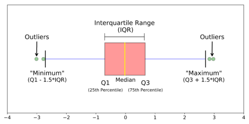
The boxplot is the simplest representation of a range and can point to outliers in your data. It is generated by plotting 5 important values: Minimum, Maximum, 25th Percentile, Median and the 75th Percentile. The Interquartile Range (IQR) is the range between the 25th and 75th Percentile, and 1.5 IQR distance is used to determine the validity of the outliers. Meaning: if a value is more than 1.5 IQR distance from the 25th or 75th percentile it is often classified as an outlier.
ACCURACY
Accuracy is the correctness of the form and content of data, for its purpose. It asks the question: to what degree does this data represent information related to an agreed-upon source?
Everyone is used to measuring accuracy daily. When you get a delivery after ordering something online, we check the content of the package against the invoice. Or skimming through the bill when you pay for your meal in a restaurant. We assess the accuracy of the data presented to us against the agreed-upon source.
The manual testing of accuracy is not a scalable solution for the large amounts of data generated by companies, but that scale also makes the assessment method more important. A somewhat simple example would be to compare postal codes to a standardized reference database, but even in such a basic operation the form already plays a part. Are you just comparing digits (1234) or including characters as well (1234 QW).
Accuracy is hard to measure metric for data quality. It involves exploratory analysis and statistics to identify trends and values that might not make sense. This requires domain knowledge, consulting an expert or running your data against trustworthy sources to determine if your findings ‘make sense’ within the context of the dataset.